Specim IQ test with Lobaria amplissima

• Agustin.Lobo@geo3bcn.csic.es
• 20221020

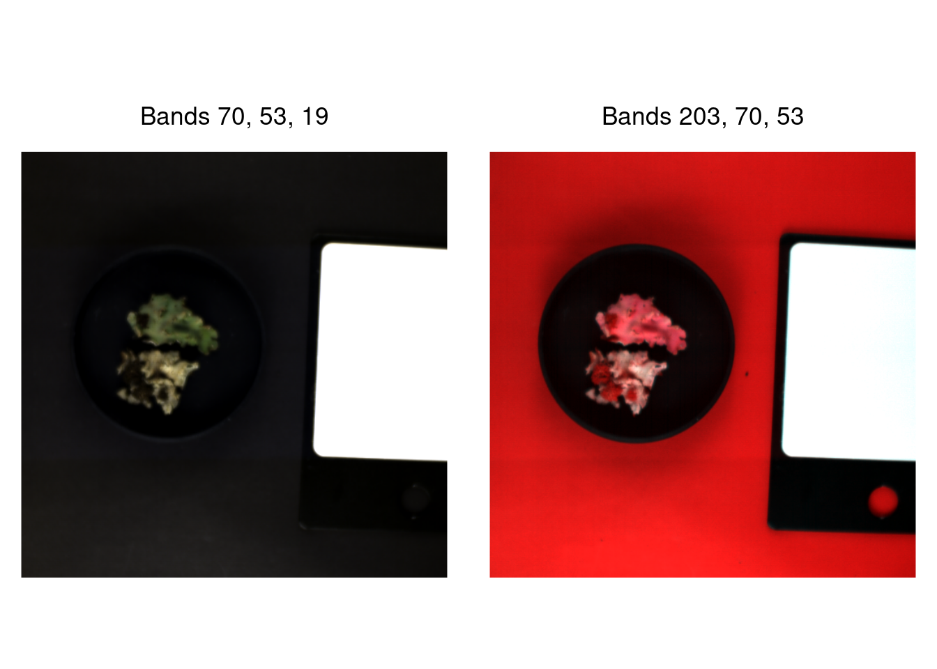
This script extracts reflectance spectra of 3 objects from a VISNIR hyperspectral image acquired with a demo unit of the Specim IQ system in HSILab premises on 20180918:

• Specim IQ white reference card.
• Lobaria amplissima (hydrated)
• Lobaria amplissima (dry)
  • Provided by joseignacio.garcia@ehu.eus

Code

defaultW <- getOption("warn")
options(warn=-1)
#Paths
RSpectDir       <- "/home/alobo/owncloudRSpect/RSpect"
datadir         <- "/home/alobo/WORK/HSI_Lab/Tests_Hypercams/SpecimIQ/SpecimIQTest_2018-09-18/2018-10-18_013"
imadir          <- file.path(datadir,"results")
vecdir          <- file.path(datadir,"QGIS/Polygons")
#libraries
library(reshape2, quietly = TRUE)
library(plyr, quietly = TRUE)
library(ggplot2, quietly = TRUE)
library(plotly, quietly = TRUE)
library(terra, quietly = TRUE)
library(tidyterra, quietly = TRUE)
library(gridExtra, quietly = TRUE)
library(directlabels, quietly = TRUE)

#Required information
load(file.path(RSpectDir,"IQbands.rda")) #Bands Specim IQ system

1. Read images and polygons

1.1 RGB image

A conventional RGB image in png format is automatically recorded by a dedicated CCD in Specim IQ. By some reason, this image is rotated vs. the hyperspectral one, so the code rotates it.

Code

options(warn=-1)
r <- rast(file.path(imadir,"RGBBACKGROUND_2018-10-18_013.png"))
r

class       : SpatRaster 
dimensions  : 645, 645, 4  (nrow, ncol, nlyr)
resolution  : 1, 1  (x, y)
extent      : 0, 645, 0, 645  (xmin, xmax, ymin, ymax)
coord. ref. :  
source      : RGBBACKGROUND_2018-10-18_013.png 
names       : RGBBACK~8_013_1, RGBBACK~8_013_2, RGBBACK~8_013_3, RGBBACK~8_013_4 

Code

#plotRGB(r, stretch="lin")
plotRGB(flip(t(r)))

1.2 Reflectance image

The reflectance image was calculated by the Specim IQ system itself using the average value of the White reference

Code

options(warn=-1)
nomref <- list.files(imadir,patt='dat')[1]
s <- rast(file.path(imadir,nomref))
s

class       : SpatRaster 
dimensions  : 512, 512, 204  (nrow, ncol, nlyr)
resolution  : 1, 1  (x, y)
extent      : 0, 512, 0, 512  (xmin, xmax, ymin, ymax)
coord. ref. :  
source      : REFLECTANCE_2018-10-18_013.dat 
names       :     397.32,   400.20,     403.09,     405.97,     408.85,     411.74, ... 
min values  : 0.09090909, 0.100000, 0.07894737, 0.07692308, 0.05797102, 0.04444445, ... 
max values  : 1.22727275, 1.172414, 1.18421054, 1.17647064, 1.17391300, 1.19780219, ... 

We display both RGB and CIR color composites with the following spectral bands:

Code

  defbands <- c(70,53,19)
  defbands2 <- c(203,70,53)
  cat("RGB")

RGB

Code

  knitr::kable(IQbands[defbands,])

	Band	Wavelength
70	Band070	598.60
53	Band053	548.55
19	Band019	449.35

Code

  cat("CIR")

CIR

Code

  knitr::kable(IQbands[defbands2,])

	Band	Wavelength
203	Band203	1000.49
70	Band070	598.60
53	Band053	548.55

Code

  crs(s) <- ""
  #suppressMessages(
  ggRad <- ggplot() + 
  geom_spatraster_rgb(data = stretch(subset(s, subset=defbands), minq=0.02, maxq=0.85)) +
    coord_fixed(ratio = 1) +
    theme_void() + theme(plot.title = element_text(hjust = 0.5)) +
    ggtitle(paste0("\nBands ", paste(defbands,collapse=", ")))
  ggRad2 <- ggplot() + 
    geom_spatraster_rgb(data = stretch(subset(s, subset=defbands2), minq=0.02, maxq=0.85)) +
    coord_fixed(ratio = 1) +
    theme_void() + theme(plot.title = element_text(hjust = 0.5)) +
    ggtitle(paste0("\nBands ", paste(defbands2,collapse=", ")))
  #)
  grid.arrange(ggRad, ggRad2, ncol=2)

1.3 Polygon vector

Significant parts of each object were interactively digitized as polygons in QGIS and used as input here.

Code

options(warn=-1)
nompoly <- "013detailed.shp"
p <- vect(file.path(vecdir,nompoly))
p

 class       : SpatVector 
 geometry    : polygons 
 dimensions  : 15, 4  (geometries, attributes)
 extent      : 121.7782, 495.9103, -354.6019, -131.6486  (xmin, xmax, ymin, ymax)
 source      : 013detailed.shp
 coord. ref. : ETRS89 / UTM zone 31N (EPSG:25831) 
 names       :    id  Name  Descript    State
 type        : <int> <chr>     <chr>    <chr>
 values      :    15 White White ref hydrated
                   1    h1        NA hydrated
                   2    h2        NA hydrated

Code

#knitr::kable(p)

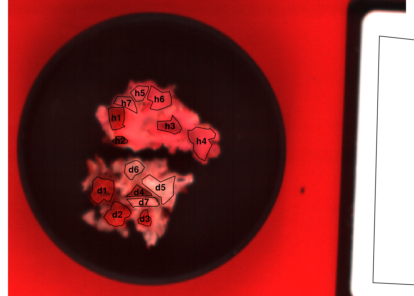
2. Make consistent geometry and display

In case the CRS is not defined (and this is the unfortunate case of Specim hdr files), R and QGIS assume, by default, different geometry for the same tiff. As a consequence, polygons digitized in QGIS do not overlay the raster image in R. The code must account for this fact, making a consistent geometry for raster and vector layer, which we confirm in the display:

Code

crs(s) <- crs(p)
ext(s) <- c(0,512,-512,0)
plotRGB(stretch(s[[defbands2]], smin=0.0, smax=0.85), ext=c(50,400,-360,-100))
#plotRGB(stretch(s[[defbands]], smin=0.0, smax=0.4), ext=c(50,400,-360,-100))
lines(p)
text(p,2,cex=0.9,font=2)

Code

#lines(p,ext=c(50,400,-360,-100)) # "ext" is not a graphical parameter
#lines(ext(c(50,400,-360,-100)))

3. Extract spectra corresponding to polygons

Using the polygons as templates, we extract the reflectance values from the hyperspectral image.

Code

options(warn=-1)
refldat.m  <- terra::extract(s, p, fun=mean, na.rm=TRUE)
refldat.sd <- terra::extract(s, p, fun=sd, na.rm=TRUE)

refldatm <- as.data.frame(t(refldat.m[,-1]))
colnames(refldatm) <- values(p)$Name
refldatm$Band <- IQbands$Band
refldatm$Wavelength <- IQbands$Wavelength
#head(refldatm)
refldatsd <- as.data.frame(t(refldat.sd[,-1]))
colnames(refldatsd) <- values(p)$Name
#head(refldatsd)

refldat <- melt(refldatm,id.vars = c("Band", "Wavelength"))
#head(refldat)
names(refldat)[3:4] <- c("Sample", "Reflectance")

a <- melt(refldatsd,id.vars=NULL)
#head(a)
refldat$sd <- a$value
refldat$State <- mapvalues(refldat$Sample, from=values(p)$Name, to=values(p)$State)
#head(refldat)

#gg1 <- plothcavspect(datainRef,title="")
#Default colors
ggplotColours <- function(n = 6, h = c(0, 360) + 15){
  if ((diff(h) %% 360) < 1) h[2] <- h[2] - 360/n
  hcl(h = (seq(h[1], h[2], length = n)), c = 100, l = 65)
}

micolor <- ggplotColours(n=24)
#scales:::show_col(micolor)
micolor <- c("White"="grey50", 
             "h3"=micolor[6],
             "h4"=micolor[7],
             "h5"=micolor[8],
             "h6"=micolor[9],
             "h7"=micolor[10],
             "h1"=micolor[4],
             "h2"=micolor[5],
             "d5"=micolor[1],
             "d6"=micolor[2],
             "d7"=micolor[3],
             "d1"=micolor[21],
             "d2"=micolor[22],
             "d3"=micolor[23],
             "d4"=micolor[24])

gg1 <- ggplot(data=refldat) +
  geom_point(aes(x=Wavelength, y=Reflectance, color=Sample),size=0.5) +
  geom_line(aes(x=Wavelength, y=Reflectance, color=Sample)) +
  #geom_errorbar(aes(x=Wavelength,ymin=Reflectance-sd, ymax=Reflectance+sd, color=Sample),
  #              width=.01,
  #              position=position_dodge(0.05)) +
  geom_text(aes(x=1010, y=Reflectance,label=Sample)) +
  xlab("Wavelength (nm)") +
  theme(legend.position = "none") +
  scale_color_manual(values=micolor) +
  ggtitle("Lobularia amplissima")
#gg1 + xlim(c(450, 1000)) + ylim(c(0,0.9)) + 
#  facet_wrap(~State) + geom_dl(aes(x=Wavelength, y=Reflectance, label = Sample), method = list(dl.combine("first.points", "last.points"), cex = 0.7)) 
gg2 <- gg1 + xlim(c(450, 1000)) + ylim(c(0,0.9)) + facet_wrap(~State) +
  geom_dl(aes(x=Wavelength, y=Reflectance, label = Sample), method = list(dl.combine("first.points", "last.points"), cex = 0.7))
ggplotly(gg2,
         tooltip=c("Band","Wavelength",Reflectance="Reflectance","Sample"))