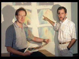
Marcelo
Assumpção to the right and
Martin Schimmel to the left
(from Pesquisa, 53,
20-27, 2000, foto by F. Cannalonga)
The P- and S-wave velocity perturbation model published in Schimmel et al. (2003) can be downloaded here.
 |
|
Marcelo
Assumpção to the right and
Martin Schimmel to the left |
A prime tool to illuminate mantle structure is seismic tomography. Although it lacks the resolving power to constrain mantle discontinuities it provides us with reconstructions of the long and intermediate scale structure. We use this tool to map the P- and S-wave velocity anomalies underneath SE-Brazil.
In the
following we list some selected figures which you can view by
clicking on the highlighted text. The results are compiled in a
publication (download
pdf.gz [6.7Mb] ).
In our publication you can find the details and more figures about
the tectonic settings, the resolution and data consistency tests.
Informations on the seismic
anisotropy, the upper mantle deformation in SE Brazil, and a
franco-brazilian portable seismic experiment are
also provided by the tectono-physics group in Montpellier.
Map with the sites of seismic stations used so far for the relative arrival time data set and gross geological provinces. The solid lines are political boundaries and the dashed lines denote the main geological provinces. Up to 15 stations have been in operation at any time to record the events from 1992 to 1999. The stations are sorted by projects or owner; `bb' and `sp' stand for broadband and short-period sensor, respectively. The short-period stations are used to increment the P-wave data set.
Histograms for the relative P- (a) and S-wave (b) residuals after correction of station elevation. The P- and S-wave data sets consist of 5367 and 4763 residuals. Core phases and first arrivals are separated by colors. A gauss-function with corresponding standard deviation and maximum count has been added for reference.
Relative travel time residuals of the direct P and S phases as function of back azimuth at stations FRMB (a), CDCB (b), BSCB (c), TRIB (d), RIFB (e), NATB (f). The symbols and error bars mark the means and standard deviations of at least four measures within a 10 deg bin centered every 5 deg.
Distribution of ray incidence angles at 400 km depth as function of back azimuths for the P- (a) and S-wave (b) data set. Every symbol corresponds to a ray. The horizontal band-shaped occurrence of incidence angles is due to the selected distance ranges. The data points cluster due to the uneven distribution of events.
Tomographic reconstructions for the P-wave phase times. The horizontal cross sections show the velocity perturbations at distinct depth levels. White lines mark the intersections with the vertical cross sections (A-A' and B-B') which are displayed in the next figure. White squares denote station sites used in the S-wave inversion. Regions with low ray-density are blacked.
Tomographic reconstructions for the S-wave phase times. The horizontal cross sections show the velocity perturbations at distinct depth levels. White lines mark the intersections with the vertical cross sections (A-A' and B-B') which are displayed in the next figure. White squares denote station sites used in the S-wave inversion. Regions with low ray-density are blacked.
The P (left column) and S (right column) velocity perturbation models are displayed as vertical cross sections A-A' and B-B'. The elevations at the Earth's surface are multiplied by 30. Shallow structure is blacked since the ray paths are almost parallel beneath the stations.
Distribution of length sum of ray segments which constrain the P- (a,c) and S-wave (b,d) velocity perturbations along the cross sections A-A' and B-B', respectively.
|
|
|
The dashed lines mark our study area (e.g. see the station map for more details, figure from Pesquisa, 53, 20-27, 2000).
|
|
|
|
P-wave velocity perturbations along the cross section A-A' (from Pesquisa, 53, 20-27, 2000). |
|
Back to my first page |